Motor Position Sensor (MPS)
Overview
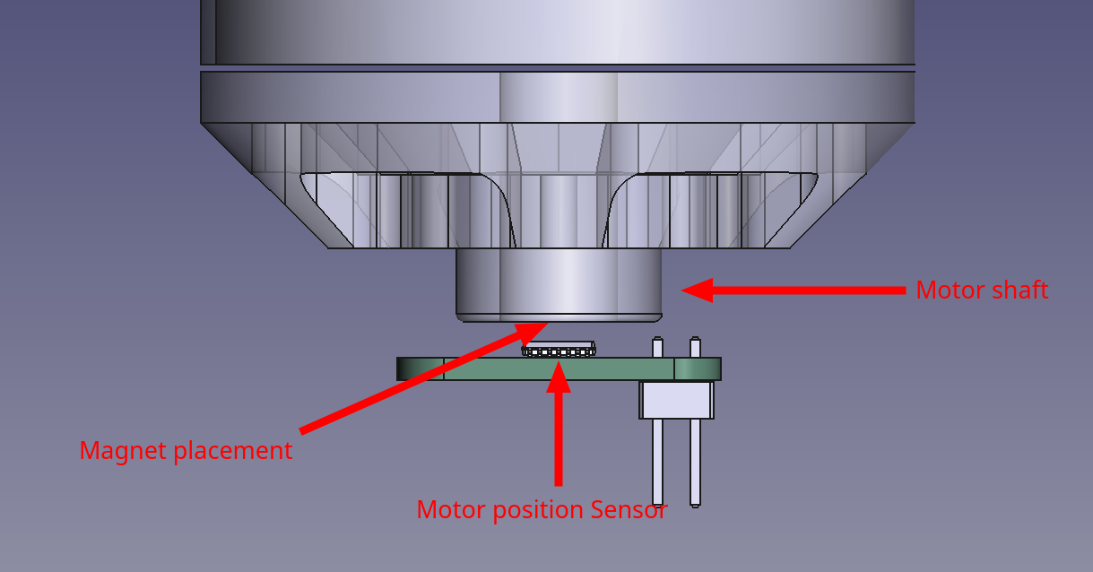
For the prototype of my BLDC Motor Controller Board a Motor position Sensor (MPS) for the feedback loop is needed during the development. This is going to be a simple small PCB that can be mounted at the axis of rotation for the motor to measure the position via a magnet. The magnetic field of the magnet is the physical parameter that is measured by the magnet. Since the magnet is mounted to the motor shaft, its direction corresponds to the mechanical position of the motor. See below the image for easier understanding.
Hardware Design
The main part of this design will be the AMS OSRAM AS5047P Magnetic Rotary Position Sensor. It features the following specifications:
- 14 bit resolution
- SPI Interface
- ABI Interface
- UVW Interace
- PWM Output
- up to 28krpm speeds
- integrated dynamic angle error compensation with low latency
- 3.3V or 5V input voltage
The datasheet can be found here for more details. I followed the manufacturer recommendations to design a compact sensor breakout board. The input voltage is selectable via the P101 and P102 solder bridges. Apart from these configuration jumpers, all functional pins of the IC are routed directly to the main interface connector.
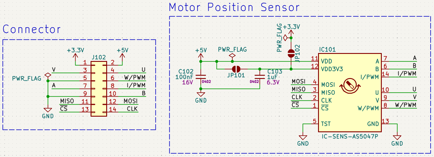
Via the P101 and P102 solder bridge it is possible to select either 3.3V or 5V for the input voltage. Apart from that all connections of the IC are routed to the connector.
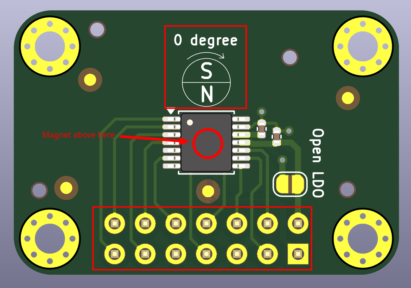
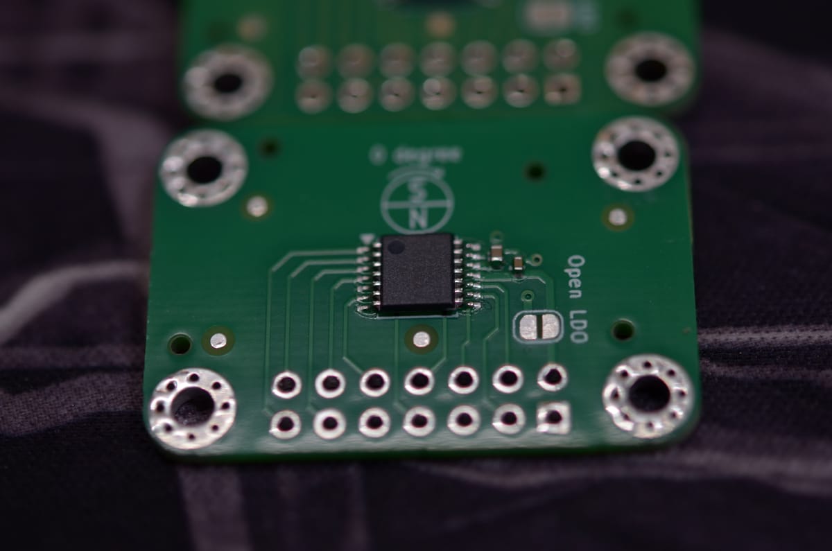
As shown in the image above the diametrically magnetized magnet has to be placed on top of the IC. Normally this is done by fixing the magnet to the motor shaft and aligning it with the IC. Also the height distance between the IC and the magnet is of importance. If this is to close the magnetic field is too strong and visa versa. After finishing the design, I ordered the PCB on JLCPCB. See below the finished boards
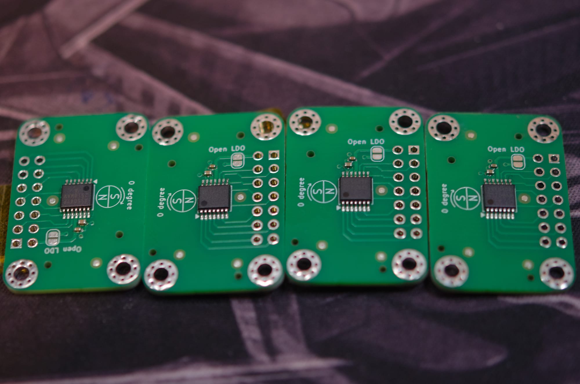
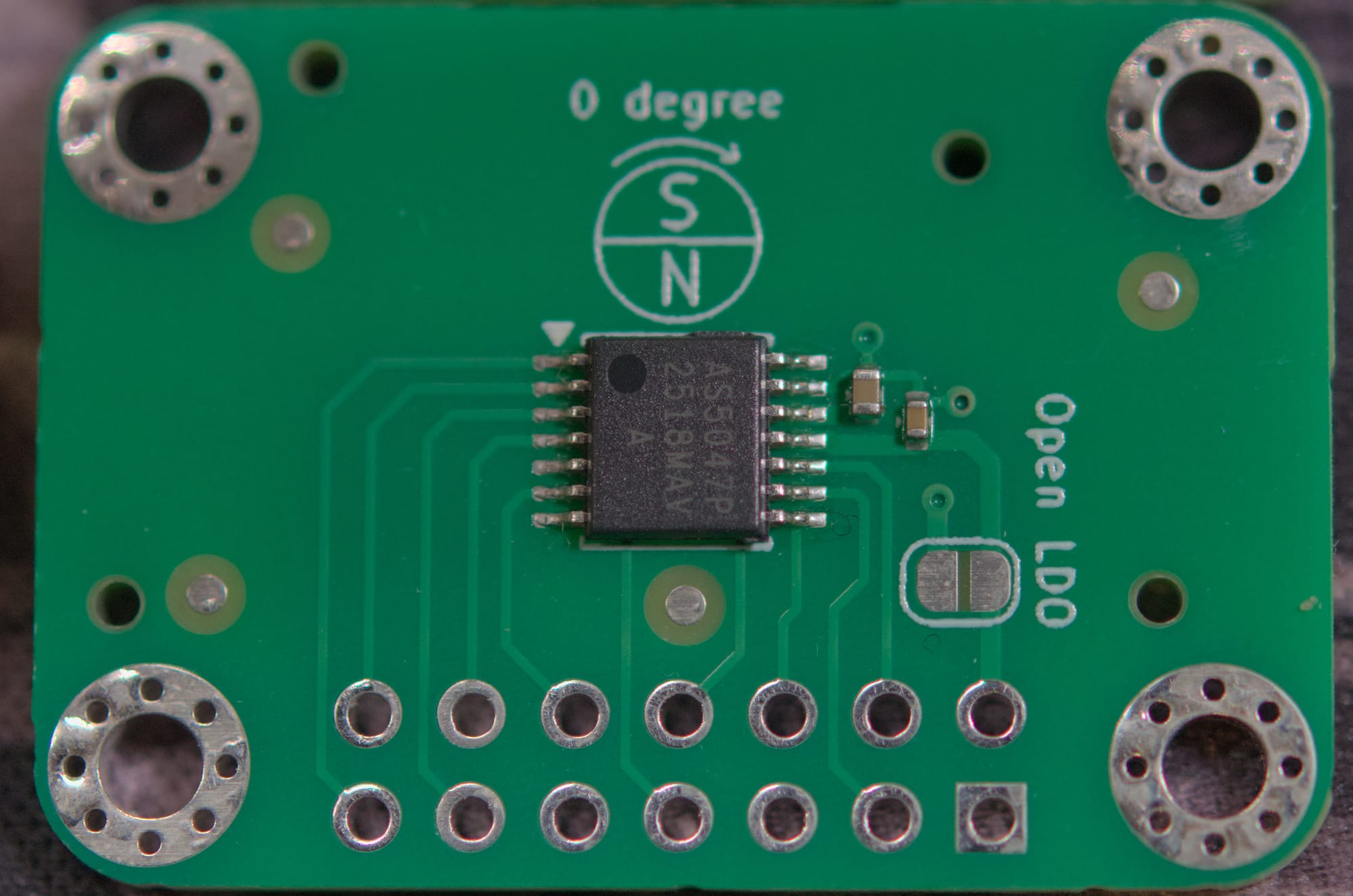
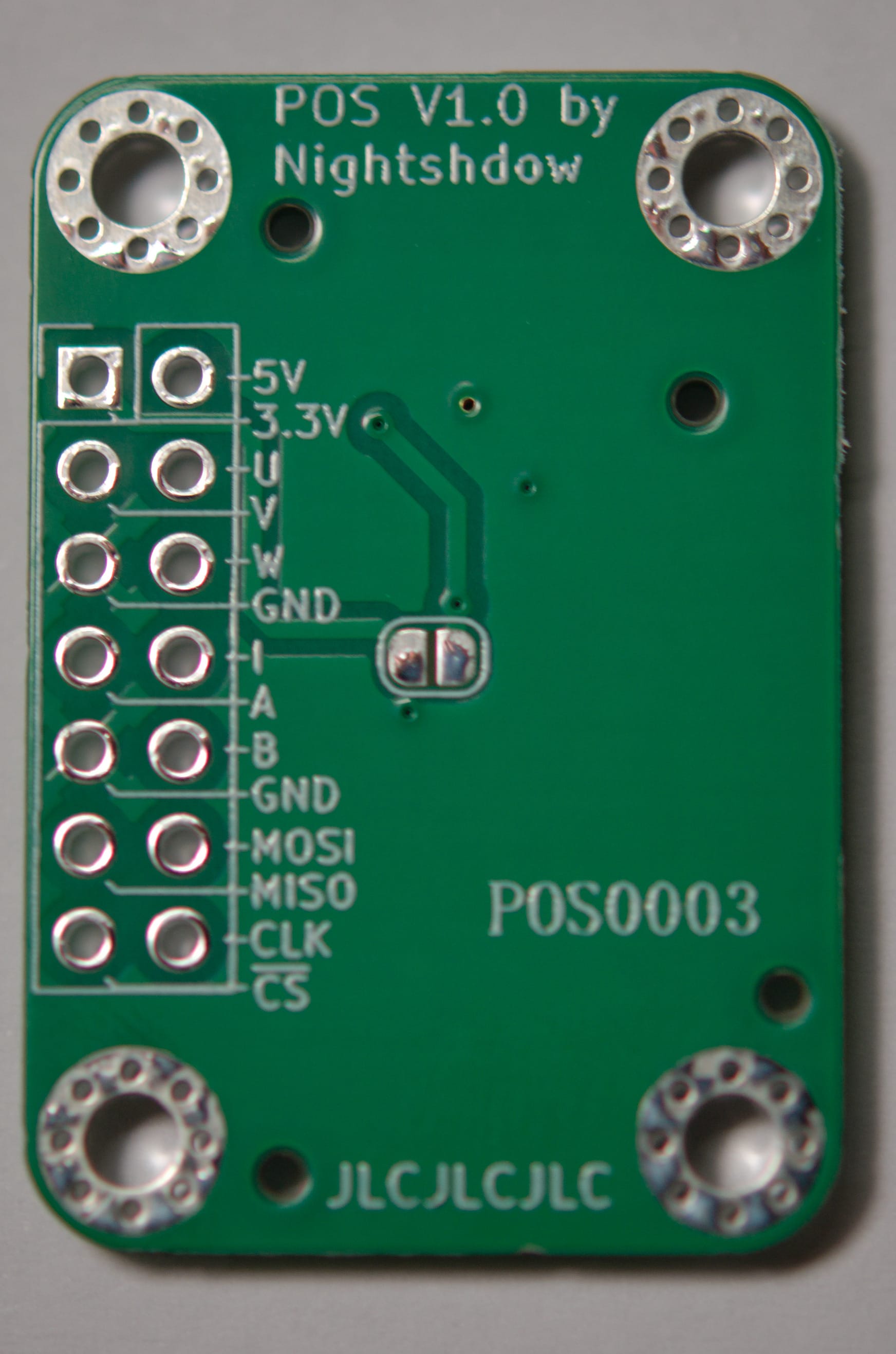
Testing
To communicate with the sensor I initially used an old custom board with an STM32F405RG that I had lying around. To program the MCU I have to use an external STLinkV2.0 for programming and the SWCLK (PA14) and the SWDIO (PA13) pins of the MCU. The interface I will be using are SPI for configuring and reading the sensor, as well as the ABI for simplicity. Later on I switch to the BLDC Motor controller board, which will get its own blog post in the future.
The next section describe the Firmware configuration via zephyr.
Clock Settings STM32
The first thing that needs verification is the clock tree configuration. The base template for this project assumed a 12 MHz external crystal, whereas my custom board uses a 16 MHz crystal. Consequently, all prescaler and multiplier values required updating. I used the STM32CubeMX software to calculate the desired prescaler values. If you want to get in to the details and do that yourself you would need to dig into the datasheet of MCU. The settings can be modified either in the <board>.overlay file or the <board>.dts file, see my final settings below:
&clk_hse {
	clock-frequency = <DT_FREQ_M(16)>;
	status = "okay";
};

&pll {
	div-m = <8>;
	mul-n = <168>;
	div-p = <2>;
	div-q = <7>;
	clocks = <&clk_hse>;
	status = "okay";
};

&rcc {
	clocks = <&pll>;
	clock-frequency = <DT_FREQ_M(168)>;
	ahb-prescaler = <1>;
	apb1-prescaler = <4>;
	apb2-prescaler = <2>;
};
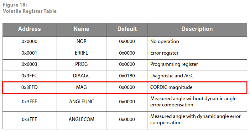
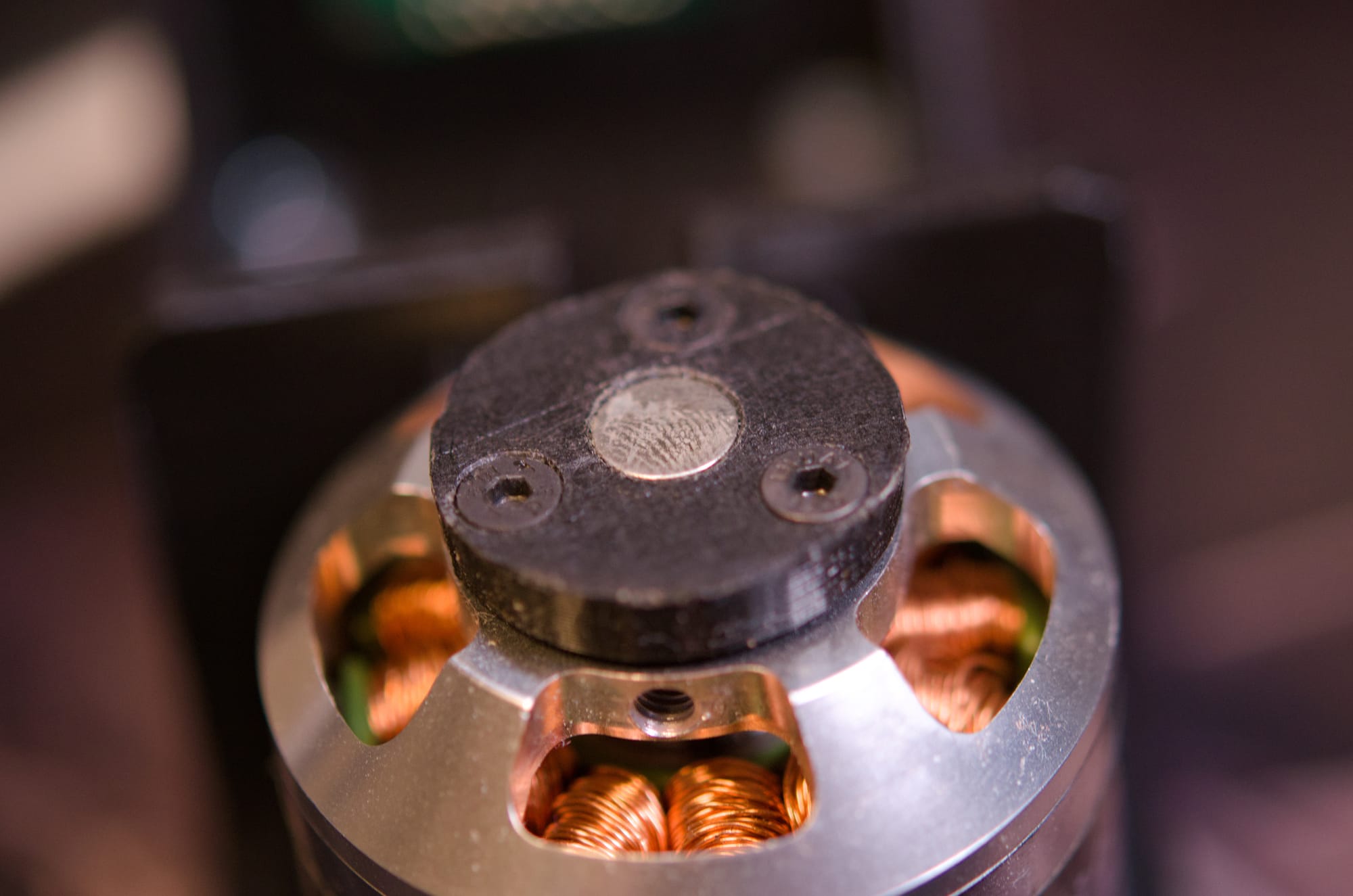
I got the SPI and the ABI interface working but I realized the BLDC Motor that I use does not have a magnet mounted. There is a section at the end of the shaft that seems magnetic and I assumed that there is a magnet built-in. But I realized that this is just the stray magnetic field of the rotor magnets. I only figured it out after reading the 0x3FFD register of the AS5047P that contains the magnetic magnitude information that this is way to low and I already had the end of the shaft pressed to the IC top :) Ups my bad!
Still with that I was able to verify that the communication and sensor reading was working. Next I ordered a correct magnet with a diametrically magnetization and designed 3D printable magnet mount. This adds a bit of length to the whole motor assembly, therefore needing to reprint the whole motor mount. Well thats what we got a 3D printer for!
ABI
Introduction
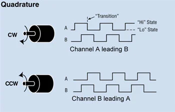
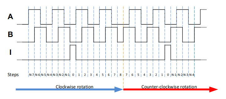
The ABI quadrature interface is a common interface for digital encoders. Quadrature encoder ABI (A, B, Index) communication uses two 90-degree out-of-phase square wave signals (A and B) to determine shaft position, speed, and direction, with the Index I providing a once-per-revolution reference. By monitoring the phase relationship (A leading B or B leading A) on the rising/falling edges of A and B, a microcontroller can increment or decrement a counter, effectively tracking incremental movement and direction, while the Index pulse resets or marks a known point, enabling precise position tracking in motor control and robotics.
STM32 Encoder support
The Stm32 has built in encoder support for different Encoder Mode. it may be necessary to switch from one encoder mode to another during run-time. This is typically done at high-speed to decrease the Update interrupt rate, by switching from x4 to x2 to x1 mode. A higher mode results in a higher resolution
See Application Note AN4014 for details.
Firmware configuration
The ABI Interface can be used with the Quadrature Encoder Sensor library that is build into zephyr.
The Timer is setup in the .dtsfile of the board like so
&timers2 {
status = "okay";
	qdec: qdec {
		status = "okay";
		pinctrl-0 = <&tim2_ch1_pa15 &tim2_ch2_pb3>;
		pinctrl-names = "default";
		st,counts-per-revolution = <2048>;
		st,input-filter-level = <1>; // default is 0
	};
};
In the main.cfile we get the sensor node and the gpio that will act as an interrupt input for the I while the two timer input are for the A and B Input.
 // ABI Interface
/* Get the devices from Devicetree */
const struct device *qdec_dev = DEVICE_DT_GET(DT_NODELABEL(qdec));
static const struct gpio_dt_spec index_gpio = GPIO_DT_SPEC_GET(DT_NODELABEL(index_pin), gpios);
static struct gpio_callback index_cb_data;

/* Callback function for Index pulse */
void index_handler(const struct device *port, struct gpio_callback *cb, uint32_t pins)
{
    /* Reset the timer counter when index pulse is detected */
    /* Note: Direct register access is often fastest for this */
    TIM2->CNT = 0;
}

void setup_encoder(void)
{
    if (!device_is_ready(qdec_dev)) {
        return;
    }

    /* Setup Index Interrupt */
    gpio_pin_configure_dt(&index_gpio, GPIO_INPUT);
    gpio_init_callback(&index_cb_data, index_handler, BIT(index_gpio.pin));
    gpio_add_callback(index_gpio.port, &index_cb_data);
    gpio_pin_interrupt_configure_dt(&index_gpio, GPIO_INT_EDGE_TO_ACTIVE);
}

double read_encoder(void)
{
	struct sensor_value qdec_value = {0};
	double precise_degrees = 0.0;
	if (sensor_sample_fetch(qdec_dev) == 0)
	{
		sensor_channel_get(qdec_dev, SENSOR_CHAN_ROTATION, &qdec_value);
		// Convert to double to see the 0.08789 degree increments
		precise_degrees = sensor_value_to_double(&qdec_value);
	}
	return precise_degrees;
}
and than we can read the sensor in the main loop
setup_encoder();
as5047p_set_abi_4096(spi3_dev, &spi_cfg, &cs_gpio);
double abi_angle = read_encoder();
Do not for get to include the sensor library at the beginning.
#include <zephyr/drivers/sensor.h>
and to enable the Sensor and the QDEC subsystem either via the Kconfig or in the prj.conf file:
CONFIG_SENSOR=y
CONFIG_QDEC_STM32=y
Measurement and Characterization
Measurement Setup
In order to verify the measurements and linearity of the measurement I created a test setup, where a stepper motor is moving the BLDC Motor. The system contains one driver board for the stepper motor and the BLDC motor controller board that is connected to the motor position sensor.
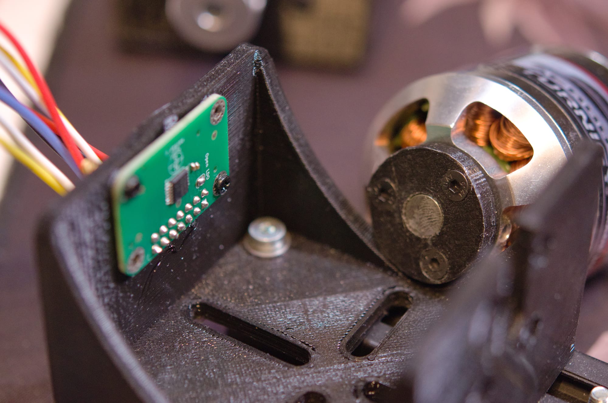
The idea is to capture the measurement of the position sensor with a fixed interval. To achieve this I decided to move the measurement to its own thread. This seems to be working for now, but I believe that I will have to learn more about threads, since it basically behaves like a normal sequential program at the moment :D. In the thread the data is measured for the SPI and the ABI Interface and stored into an array. After all measurements are done the array is printed in a .csv format to the UART, where I can than can store it and further analyse it in python. I can modify the array size and the trigger interval for the measurement. In the end I opted for 2 rotations in one direction and than 2 rotations in the other direction. With that I should get at least one full rotation with a constant speed. The acceleration and deacceleration should happen in the first and last half of one rotation. To sync the movement of the stepper controller board with the measurement of the motor controller board I used an interrupt to signal that the movement started. This triggers the start of the measurement on the motor controller board.
Initial Measurement
After the first successful measurement I plotted the data in python with the help of the matplotlib library.
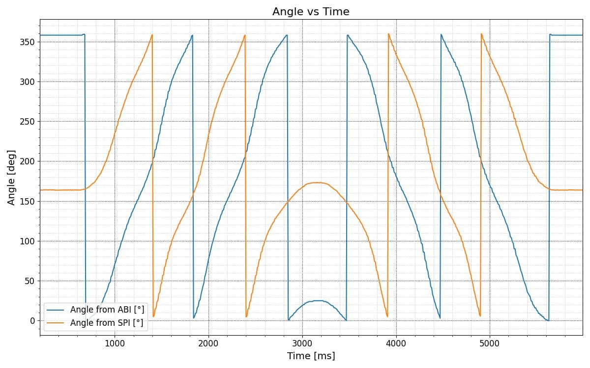
The obvious thing to notice is that the ABI and SPI reading are out of sync. Apart from that there is a clear non-linearity visible. Things to consider the stepper motor uses a ramp up at the start and end, but in between the motion should be almost linear. Since I got in touch with an Allegro MPS at work that had built in linearization, I though I might be able to implement this for my sensor in the firmware.
Linearization
Before starting with the linearization I had a better look at the measured data.
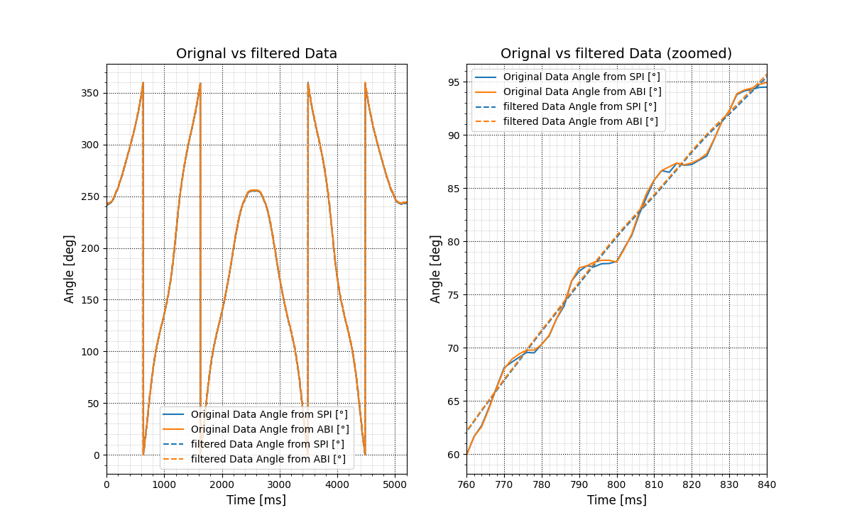
As can be seen in the zoomed in plot section the original data is accompanied by an oscillation/vibration, which is also audible during the test. I tried to reduce the speed of the stepper motor during the test and also to make the coupling between the BLDC motor and the stepper motor better with no success. After removing the BLDC motor and only spinning the stepper motor the vibration was gone, therefore I assume that the main issue here are the magnetic properties of the BLDC which is due to the cogging torque. This is caused by the permanent magnets of the rotor and the teeth of the stator iron core. To mitigate this issue I decided to implement a filtering of the measurement data before calculating the error correction factors.
Assumptions
I used an ideal linear curve as my reference signal for the calculations. As discussed before, I only isolated the middle section of the measured signal for both directions. Because the stepper motor requires time to ramp up to speed and slow down, these acceleration and deceleration phases introduce non-linear velocity profiles at the boundaries. To prevent this from skewing the calibration, the ramping regions were entirely excluded. I performed a linear fit strictly across the constant velocity window, mapping a straight line directly from the entry point to the exit point of this stable region to act as the true mechanical reference baseline. This process is visualized in the plots below.
Linear interpolation
Based on the Allegro Linearization described here: https://www.allegromicro.com/en/insights-and-innovations/technical-documents/hall-effect-sensor-ic-publications/an296161-linearization-aas330x1 I create a linear optimization based on 32 measurements. My first attempt resulted in bad accuracy for the linear interpolation. I later figured out that this was to a bad polynomial fit (only 5 coefficients) of the error as shown below. Based on this bad fit I deceided to try a harmonic fit as well.
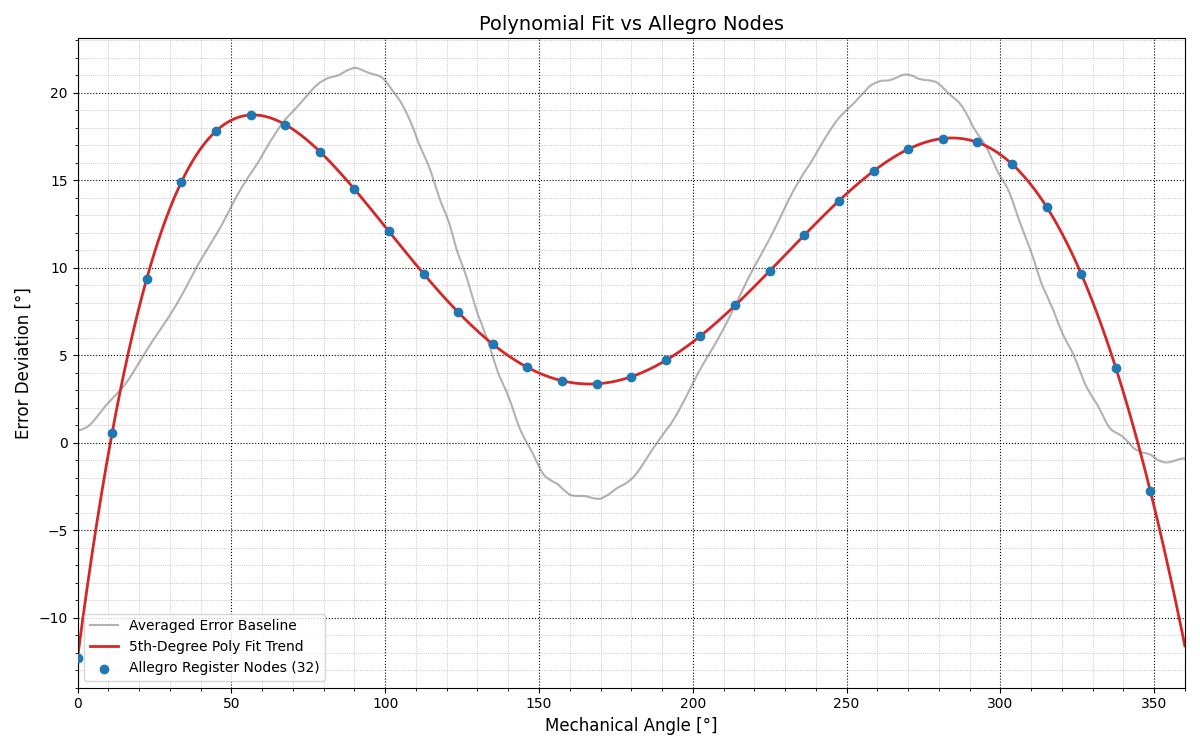
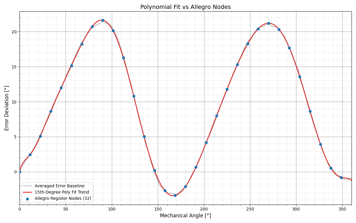
After imporving the polynomial fit by increasing the coeefficients to 15 the linearization results where also much better and can be seen in the following diagrams.
Harmonic optimization
Based on the observed measurement it seems like a harmonic component is overlayed. For this reason I decided to also try a harmonic based optimisation
The optimization problem can be expressed as:
$$ \min_{\mathbf{c}} \Vert{}\mathbf{A}\mathbf{c} - \mathbf{e}\Vert{}_2^2 $$
Where the error function for a single measurement angle \theta_n (in radians) is modeled by the equation:
$$ e_n = c_0 + \sum_{i=1}^{4} \left( c_{2i-1} \sin(i \theta_n) + c_{2i} \cos(i \theta_n) \right) $$
Results
Below we can see the results for the linear and harmonic linearization.
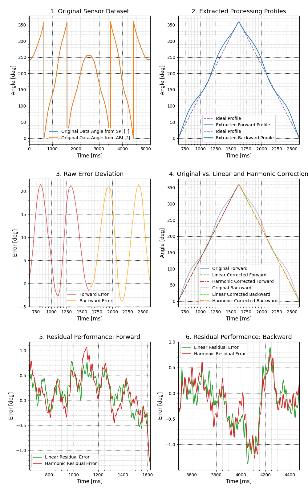
We can see a comparison of the linear and the harmonic Correction in the 4th subplot and the residual errors in the 5th and 6th. Based on these results both seem to be yield similar performance, at least for the measured signal. To verify the results next I used the calculated correction factors from the python script and implemented the correction process in the firmware.
Implementation of the correction in Zephyr
For testing I implemented both correction calculations in Zephyr.
Linear
// 32-segment lookup table values
static const float32_t lut_corrections[32] = {
0.000404,
-2.431294,
-5.089021,
-8.636107,
-11.983723,
//....
}

float32_t apply_linear_correction(float32_t raw_angle_deg) {

	// CMSIS-DSP linear interpolation uses an instance structure
	arm_linear_interp_instance_f32 S;
	S.nValues = 32;
	S.x1 = 0.0f; // First point location
	S.xSpacing = 11.25f; // 360 / 32 elements
	S.pYData = (float32_t *)lut_corrections;
	// Evaluate the correction factor at the current raw position
	float32_t correction = arm_linear_interp_f32(&S, raw_angle_deg);
	// Apply correction and wrap to 0-360
	float32_t corrected_angle = raw_angle_deg + correction;
	if (corrected_angle >= 360.0f) corrected_angle -= 360.0f;
	if (corrected_angle < 0.0f) corrected_angle += 360.0f;

	return corrected_angle;
}
Harmonic
// Coefficients generated by your harmonic optimization script
#define NUM_HARMONICS 4
static const float32_t dc_offset = 9.751351;
static const float32_t sin_amps[NUM_HARMONICS] = {
-0.520884,
2.514248,
-0.536992,
1.135013
}; // 1st, 2nd, 3rd, 4th harmonic

static const float32_t cos_amps[NUM_HARMONICS] = {
1.156572,
-11.194734,
-0.022124,32,
0.428432
};

float32_t apply_harmonic_correction(float32_t raw_angle_deg) {
	// Convert base angle to radians for CMSIS functions
	float32_t theta_rad = raw_angle_deg * (PI / 180.0f);
	// Initialize error calculation with the DC offset parameter
	float32_t estimated_error = dc_offset;
	// Evaluate the Fourier series up to N harmonics
	for (int i = 1; i <= NUM_HARMONICS; i++) {
		float32_t n_theta = (float32_t)i * theta_rad;
		// Fast CMSIS-DSP lookup functions
		float32_t sin_val = arm_sin_f32(n_theta);
		float32_t cos_val = arm_cos_f32(n_theta);
		estimated_error += (sin_amps[i-1] * sin_val) + (cos_amps[i-1] * cos_val);
	}
	// Subtract the estimated error curve from the raw input measurement
	float32_t corrected_angle = raw_angle_deg - estimated_error;
		// Wrap tracking window boundaries to (0, 360) range
		if (corrected_angle >= 360.0f) corrected_angle -= 360.0f;
		if (corrected_angle < 0.0f) corrected_angle += 360.0f;
		return corrected_angle;
}
Result in Firmware
See below the output of the correction in comparison to the original measurement for the SPI and ABI reading.
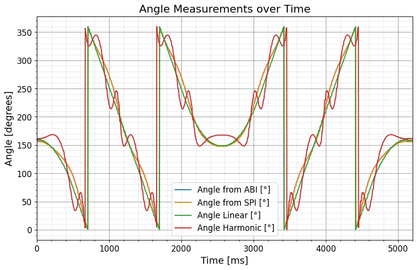
As can be seen the harmonic correction did not work. I tried a different implementation in C as well. To verify if this was an implementation issue on my side I injected the original correction factor into the python script while using the new data, which resulted in the output below.
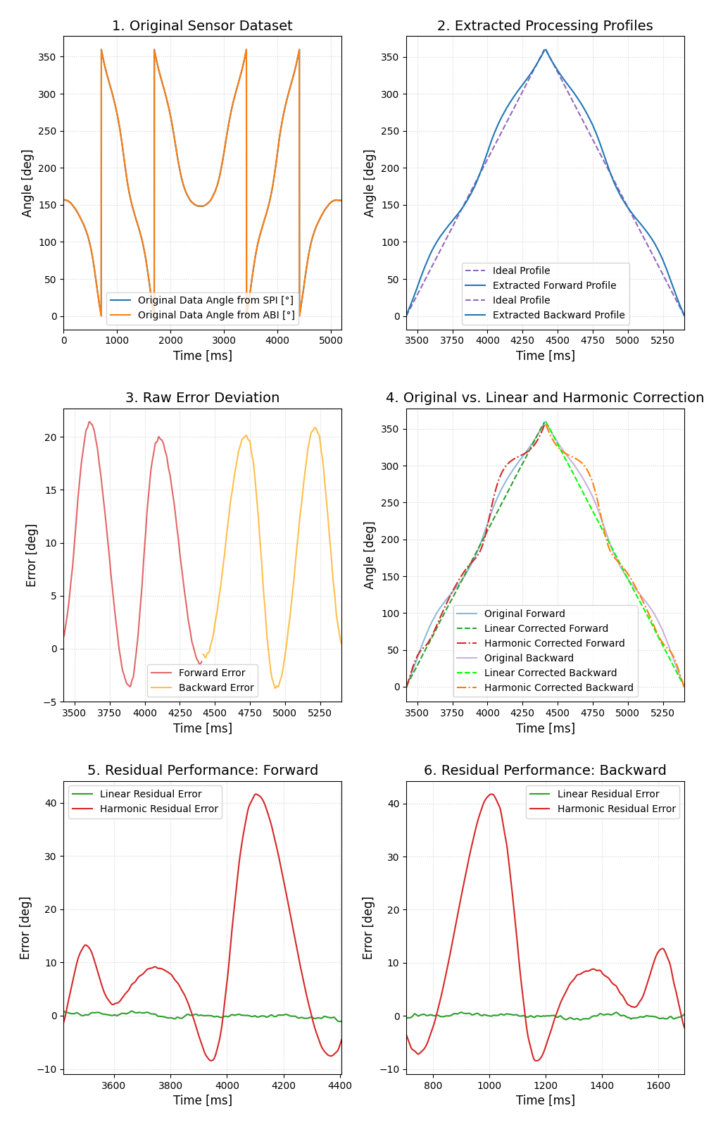
The actual implementation in firmware revealed that the harmonic correction failed, resulting in large tracking errors.Further analysis indicated that the optimization function is strictly tied to the initial motor startup position. Altering the mechanical starting point introduces a constant phase shift \phi to the measurement angles, altering the absolute coordinates:
$$ \theta'_n = \theta_n + \phi $$
Substituting this phase shift into the error model shows why the predefined harmonic coefficients break down under variable starting conditions:
$$ e_n = c_0 + \sum_{i=1}^{4} \left( c_{2i-1} \sin(i (\theta_n + \phi)) + c_{2i} \cos(i (\theta_n + \phi)) \right) $$
Well I could have checked this beforehand, which would have made my life a lot easier. But hey I learned something along the way, so who cares!
Because the harmonic model lacks phase invariance across different power cycles and startup positions, I removed the harmonic optimization code from the firmware. The linear lookup table interpolation remains the chosen method for deployment since it relies purely on absolute position values mapped to specific segments. Therefore I will be using the linear correction. With this I am able to mitigate the errors due to misalignment and other error components. The downside is that I have to do this calibration process for each individual assembly. Still I am pleased with the results and looking forward to using the MPS and the correction method in the BLDC feedback loop for the motor controller board. See you next time!